Mapping_Standards_Version_1.16

Mapping Standards and Data Quality

for the IUCN Red List Categories and Criteria

!"#$%&'()*)+(

,-"./"01"#(23)45(

6#".7#"8(19(:"8(;%$/(<"=>'%=7?(@&#A%'B(C#&D.

Contents

Contents 2

1 Spatial data and the IUCN Red List 4

1.2 Reasons for a distribution map 4

2 What distribution data are needed for Red List assessments? 5

2.1 Textual description and SIS 5

2.2 Countries of occurrence (COO) 6

2.3 Distribution map 6

3 Taxon and system differences 7

3.1 Terrestrial and marine taxa 8

3.2 Inland water taxa (Freshwater) 8

4 Attributes for distribution maps 9

4.1 Polygon and point data 9

4.1.1 Required polygon and point attributes 9

4.1.2 Recommended polygon and point attributes 11

4.2 Point data 13

4.2.1 Optional point data 13

5 Coding of Presence, Origin and Seasonality for distribution maps 14

5.1 Presence codes 14

5.2 Origin Codes 16

5.3.1 Presence, Origin and Seasonality quick reference 17

6 Spatial information in SIS 18

6.1 Countries with multiple distribution codes in the spatial data 18

7 Extent of occurrence (EOO), area of occupancy (AOO) 19

7.1 Extent of occurrence (EOO) 19

7.2 Area of occupancy (AOO) 21

8 Generating a distribution map 23

8.1 Software and formats 23

8.2 Tools 24

8.3 Standard GIS layers / basedata 24

8.4 Mapping consistency 25

8.5 Sensitive species guidelines 26

9 What will happen to your map data? 27

9.1 Countries of occurrence (COO) data 28

9.2 Legend combinations from distribution codes 28

10.0 Updates regarding Spatial Data 28

10.1 Presence Codes (last updated 2014) 28

10.1.1 Implications of updated Presence for existing spatial data 28

10.2 Origin code Assisted Colonisation (last updated 2016) 29

10.3 Legend Update (last updated 2016) 29

11 Abbreviations, acronyms and definitions 29

1 Spatial data and the IUCN Red List

Spatial data are a key component of the IUCN Red List from the criteria that measure

species distributions to spatial filtering on the Red List website, and detailed analysis of

distribution maps to support conservation. This document provides an overview of the

different elements of spatial data on the Red List and outlines what kinds of spatial data

Red List assessors are required to provide with each assessment, along with relevant

formats and standards, with a particular focus on the distribution map.

1.1 Why spatial data are required

Spatial data are some of the most highly sought-after data on the IUCN Red List as they

are crucial information for conservation planning. Each assessment should provide

spatial data in some form.

Spatial data are essential for supporting assessments done under IUCN Red List Criteria

B and D2 (and arguably also for demonstrating that the thresholds for these criteria are

not met).

All Assessors should produce the most accurate depiction of a taxon’s distribution based

on their knowledge and the available data, in a format that is considered most

appropriate for that taxon to inform conservation action. This is used to generate the

maps displayed on the IUCN Red List website.

1.2 Reasons for a distribution map

A key component of spatial data is the distribution map (see section 2.3), which is a

depiction of a taxon’s distribution for communication and/or conservation planning

purposes; it may not equate to either the spread of extinction risk (i.e., extent of

occurrence) or the occupied range area (i.e., area of occupancy) as defined by the IUCN

Red List Categories and Criteria.

There are three main reasons for creating a distribution map for taxa being assessed for

the IUCN Red List:

● Informing Red List assessments: Distribution maps can help to inform Red List

assessments by supporting calculations of some parameters used in the assessment

process, such as the extent of occurrence (EOO).

● Helping to identify conservation priorities: Spatial data can be used for analyses,

which can inform conservation planning and policy, identify priority areas for

conservation, identify gaps in scientific knowledge, and help inform business

decisions (e.g., where not to expand development).

● Visual representation: A distribution map provides a visual representation of a

taxon’s distribution. By combining spatial data for many taxa and analysing these

alongside other Red List data (e.g., Red List Category), informative maps can be

prepared to, for example, highlight areas with high numbers of threatened species.

2 What distribution data are needed for Red List assessments?

Spatial data are required to support all new IUCN Red List assessments, except for taxa of

unknown provenance (e.g., some Data Deficient taxa) (see Annex 1 of the Rules of

Procedure). Spatial information can be grouped into three elements:

1. Textual description of the distribution (Geographic Range Information).

2. Countries of occurrence (COO), coded by presence, origin and seasonality.

3. A distribution map that represents the best available depiction of the historical,

present and projected distribution of a taxon – also coded by presence, origin and

seasonality.

2.1 Textual description and SIS

A concise narrative of currently available information on the geographic range of the

taxon is required supporting information for all taxa that are not assessed as Least

Concern (Table 2 of Annex 1 of the Rules of Procedure). For taxa that are particularly

sensitive to collecting or hunting, it is prudent to avoid providing information that allows

people to see exactly where the taxon can be found, but a less precise summary should

be provided.

It is important to provide documentation in the assessment on how the map was created

and the data sources/methods used (in SIS (Species Information Service) this is recorded

within the Geographic Range text and the Map Status fields).

It is mandatory to fill the Map Status field in SIS, which can take the values below:

• Done – the map has been completed and will be provided as part of the

assessment, and will be published.

• Missing – the map is missing and needs to be located. A submitted assessment

with this status will not be published.

• Incomplete – the map will be provided, but it is known not to be complete e.g.

there wasn’t enough information to map certain part of the range. It will be

published. A reason will need to be provided in the justification box in SIS.

• Not Possible – making a distribution map for the species is not possible e.g.

distribution is only known at coarse country level, or for Data Deficient species

where distribution is not known. A reason will need to be provided in the

justification box in SIS. A submitted assessment with this status can be published

without a map.

See the Supporting Information guidance document on the IUCN Red List website for

more information.

2.2 Countries of occurrence (COO)

The countries where the taxon occurs must be entered into SIS, with the appropriate

distribution codes for Presence, Origin and Seasonality (see section 5.0 for an

explanation of the Presence, Origin and Seasonality codes). Assessors need to ensure

that the Countries of Occurrence (COO) on the spatial map are consistent with those

listed in SIS. In future, there may be some functionality to help automate this process –

but it will still be the Assessor’s responsibility to ensure that the COO in SIS correspond

to those on the spatial map. See section 6.0 (Spatial information in SIS) for more

information.

To minimize inconsistencies between SIS and the distribution map, it is also crucial to

make sure that the appropriate recommended country basemap dataset is used (this is

available from the IUCN Spatial Data Resources page on the IUCN Red List website).

2.3 Distribution map

We encourage Assessors to provide the best possible map they can make (i.e., as

accurate as possible considering the available data) to better support/inform

conservation planning and actions. To ensure efficiency and ease of data management,

it is preferable to submit the representation of the geographic range (i.e., distribution

map data) in the following formats (can be one or a mixture of the below formats):

1) Occurrence Data (Point/s): The historical, present and projected occurrence of

a taxon is referenced by a set of coordinates known as a point locality.

2) Polygon Data: The historical, present and possible distribution of a taxon’s

occurrences is referenced by a polygon or set of polygons.

3) Basins: The historical, present and possible distribution of a taxon’s occurrences

is referenced by a basin (HydroBASINS) or a set of basins. Basins is used as a

short term for HydroBASINS – more information can be found here.

The recommended projection is WGS84 (World Geodetic Survey 1984).

The distribution map (commonly referred to as “limits of distribution” or “field guide”

map) aims to provide the current known distribution of a taxon within its native,

historical and introduced range. The limits of distribution are determined by using

known occurrences of the taxon, along with knowledge of habitat, elevation limits, and

other expert knowledge of the taxon and its range. In most cases the distribution is

depicted as polygons. Essentially, a polygon displays the limits of a taxon’s distribution,

and is intended to communicate that the taxon probably only occurs within the polygon,

but it does not mean that it is distributed equally within that polygon or occurs

everywhere within that polygon.

Options 1,2 and 3 above are not mutually exclusive; an assessment can be supported by

a combination of occurrence data and polygons. Independent of method used, a

minimum set of attribute data (metadata) should be provided; the attribute information

is described further in section 4.0.

3 Taxon and system differences

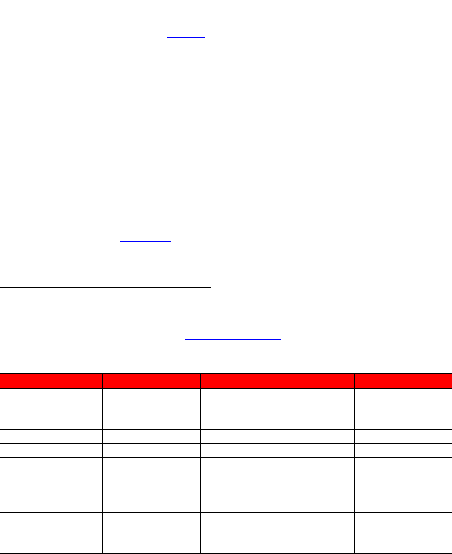
Table 1 shows the preferred approaches (i.e., polygons, basins, points) for different

taxonomic groups and systems. These are not intended to be strict rules; for any deviations,

please contact the GIS team within the IUCN Red List Unit.

Table 1: Preferred approaches by taxa and by system.

Group

Terrestrial

Inland Water

Marine

Mammals

Points Polygons

Polygon informed by basin

Points; Polygons

Birds

Points; Polygons

Polygon informed by basin

Points; Polygons

Amphibians

Points; Polygons

Polygon informed by basin

N/A

Reptiles

Points; Polygons

Polygon informed by basin

Points; Polygons

Fishes

N/A

Points; Basins

Points; Polygons

Molluscs

Points; Polygons

Points; Basins

Points; Polygons

Odonata and

ecological

equivalents

Basins

Points; Basins

Points; Polygons

Crustaceans

Points; Polygons

Points; Basins

Points; Polygons

All other

invertebrates

Points; Polygons

Points; Basins

Points; Polygons

Plants*

Points; Polygons

Points; Basins

Points; Polygons

Fungi

Points; Polygons

N/A

* For plants, most experts collect point locality data but do not produce polygon maps (with some exceptions,

e.g., cacti). For assessments that are accompanied by points only, it is recommended that a Minimum Convex

Polygon (MCP) map (equivalent to the maximum EOO as defined in this document) is produced, where

possible and appropriate, for display on the IUCN Red List website along with the points, and which could

also be used for analysis purposes.

** “Inland Water” includes taxa occurring in freshwater, brackish and estuarine habitats. Wherever it applies,

points should be provided if more specific location of the taxa within the basin is known.

3.1 Terrestrial and marine taxa

A taxon’s distribution can be provided either as point or polygon data. For polygon,

areas of unsuitable habitat, climate or physical geography (e.g. altitude, bathymetry,

hydrology) should be removed to provide a refined range.

3.2 Inland water taxa (Freshwater)

The distribution map of inland water taxa is highly recommended to be made using the

official HydroBASINS sub-basin layer, available from the IUCN Spatial Data

Resources page on the IUCN Red List website. HydroBASINS are available in different

resolutions (size of sub-basins), with the smaller sub-basins (e.g., levels 10 and 12)

being nested within larger sub-basins (e.g., level 8). The appropriate resolution to use

will depend on the level of knowledge of the taxon as well as size of its distribution

range.

For inland water taxa, as with other groups, the distribution map should represent the

best possible representation of the distribution. For those inland water taxa with

distributions more restricted than the finest scale HydroBASINS layer (e.g., the location

of a cave or small wetland to which a taxon is restricted), the range should be mapped

as a polygon reflecting the specific distribution, rather than generalising to the finest

scale HydroBASIN layer. By using a coarser HydroBASIN layer, (e.g., where a taxon

only occurs at an edge of the basin or only in a main channel), this will inflate the MCP

(see EOO description below).

If point data are being provided for inland water taxa, assessors are strongly encouraged

to provide the corresponding HydroBASINS data as well. HydroBASINS data are used

in multiple projects coordinated by the IUCN Freshwater Biodiversity Unit and

providing these data will ensure the maps are included as part of large scale analyses

using this type of spatial data.

More detailed information about mapping of inland water taxa can be found on the

IUCN Spatial Data Resources page on the IUCN Red List website.

4 Attributes for distribution maps

For the distribution map, there is a list of data attributes which must be recorded for both

polygon and point data. These attributes help describe the taxon’s distribution. Please refer

to the standards for Points and Polygons on the Spatial Resources Page of the IUCN Red

List website.

Tables 2 and 3 list the standard attributes for spatial data; the codes used to indicate

Presence, Origin and Seasonality. These codes are also used to create legends for the

distribution map (see section 9.2).

Please note that only the Required and Recommended fields are displayed in Tables 2 and

3 – more information on these can be found on the Spatial Resources Page.

The spatial attributes field names are limited to 10 characters in order to match the

Shapefile format (i.e. the Shapefile format does not allow field lengths of greater than 10

characters).

4.1 Polygon and point data

4.1.1 Required polygon and point attributes

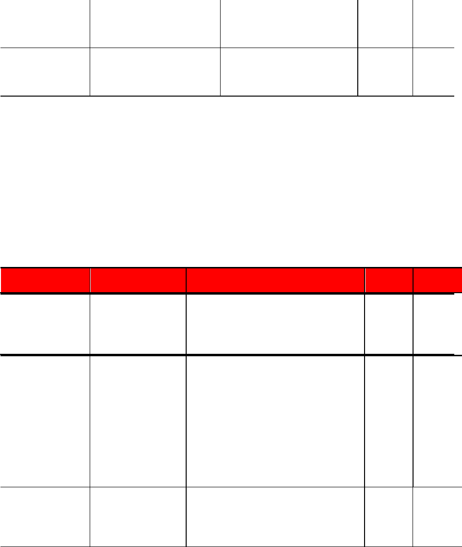
Table 2 lists the Required attributes for polygon and point data. Note that some of

these attributes are taxon dependent: these are the attributes described as “[Required

(if relevant)]” in the Description column. For example, polygon depicting the

distribution of a subspecies (e.g., Panthera leo ssp. persica) the subspecies attribute

field must be completed.

Table 2: Required attributes for polygons and points (see * which indicates which

fields apply to polygons or points)

Field

Description

Notes

Polygons

/Basins

Points

ID_NO

Unique ID for the Taxon

Species taxon ID in SIS

HYBAS_ID

HydroBASIN ID *

Only required if HydroBASINS

have been used for mapping

the data

BINOMIAL

Scientific name of the species

This must match the

corresponding field in SIS

PRESENCE

Is/Was the species in this area

See Presence coding

ORIGIN

Why/ How the species is in

this area

See Origin coding (default is “1”

if not indicated)

SEASONAL

What is the seasonal

presence of the species in the

area

See seasonal coding (default is

“1” if not indicated)

COMPILER

Name of the individual/s or

institution responsible for

generating the taxon

distribution, if not IUCN.

Names should be given in full

(e.g., John Smith; NatureServe;

World Conservation Monitoring

Centre, etc). If not indicated,

this will default to “IUCN”

YEAR

Year in which the taxon

distribution was mapped or

compiled, or modified

If not indicated, this will default

to the current year

CITATION

Individual/s or institution

responsible for providing the

data

This must be the same

throughout the file, and is how

the data points will be credited

on the IUCN Red List. If not

indicated, this will default to

"IUCN (International Union for

Conservation of Nature)"

DEC_LAT

The graphical latitude in

decimal degrees, e.g. -41.097

Positive values are North of the

equator; negative values are

South of it. Legal values lie

between -90 and 90.

DEC_LONG

The geographical longitude in

decimal degrees, e.g. -121.25

Positive values are East of the

Greenwich Meridian; negative

values are West of it. Legal

values lie between -180 and

180

SPATIALREF

The ellipsoid, geodetic datum

or spatial reference system

(SRS) upon which the

geographic coordinates given

in dec_lat and dec_long as

based. Data is preferred in

WGS84. If Blank, will default

to WGS84

For e.g., EPSG:4326; WGS84;

NAD27; Campo Inchauspe;

European 1950; Clarke 1866.

SUBSPECIES

Subspecies Name/Epithet

[Required if relevant]

Only if assessed at the

subspecies level. This must

then match the corresponding

field in SIS. For e.g., “Panthera

leo ssp. persica”

SUBPOP

Subpopulation Name/Epithet

[Required if relevant]

Only if assessed at the

subpopulation level, for e.g.,

“Chelonia mydas Hawaiian

subpopulation”

DATA_SENS

Flags up whether or not the

polygon distribution/data

point is sensitive. This is most

likely to be the case if the

Yes or No field. If “Yes”, then

the field “Sens_comm” should

be completed

polygon/s or point effectively

correspond to individual

localities. [Required if data is

sensitive]

SENS_COMM

Comments on why the data

are considered sensitive

[ Required if DATA_SENS is

‘Yes’ ]

Max 255 characters.

• HydroBASINS: If basins have been used to provide distribution data then the

HYBAS_ID, which is the unique identifier of that HydroBASIN where the taxon

has been mapped, should also be provided

4.1.2 Recommended polygon and point attributes

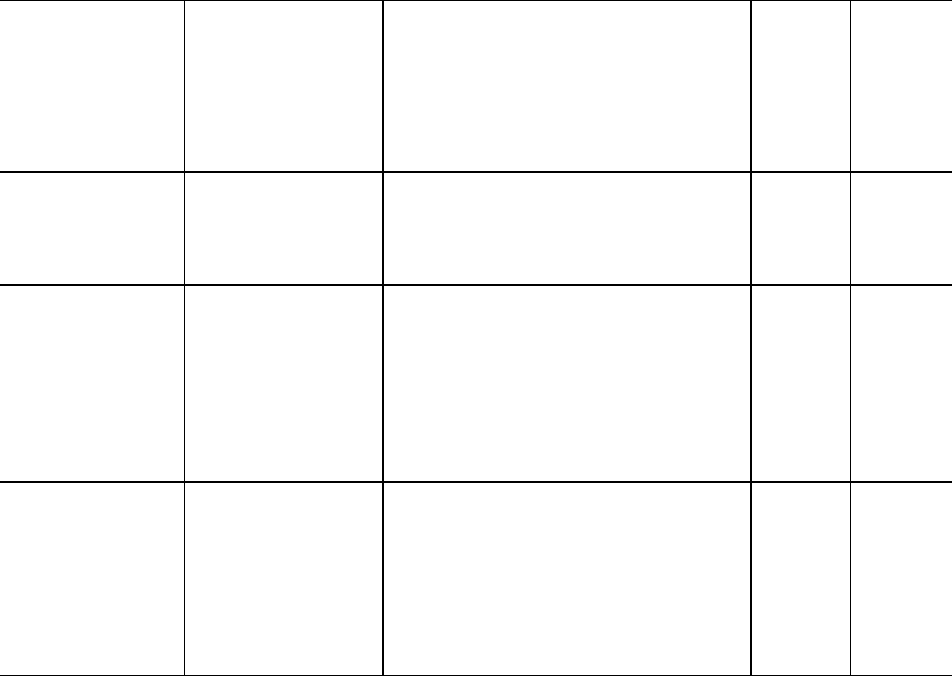
The Recommended attributes are listed in Table 3. Although they are not absolutely

required, these attributes should be recorded whenever this information is available,

so we encourage effort being made to enter the relevant information into these fields

as much as possible.

Table 3: Recommended attributes for polygons and points

Field

Definition

Notes

Polygon/

Basin

Point

EVENT_YEAR

The four-digit year in

which the Event

(object or

observation)

occurred -

For e.g., 2008

SOURCE

Provide source of

distribution range /

point data

Relates to the primary source used to

compile each polygon or point, especially

in a recently published range map, or a

set of point data. If compiled in a

workshop, or compiled from numerous

sources, then field may be left empty.

References should be in the format

“AuthorX and AuthorY, date” and the

reference should be in the corresponding

IUCN Red List assessment [max 255

characters]

CATALOG_NO

An identifier

(preferably unique)

for the record within

the data set or

collection

Name of the museum or herbarium and

the specimen number

DIST_COMM

Distribution

comments that refer

directly to the

polygon or point

Examples include whether the polygon

represents the type locality, names of

protected areas or geographical features,

and so forth. May also include specific

notes on presence, origin or seasonality

[max 255 characters]

ISLAND

Name of the island

where the polygon

or point is on

This relates mainly to very small islands or

atolls (e.g. Midway Atoll; Meemu Atoll;

Bohol)

TAX_COMM

Taxonomic

comments that refer

directly to the

polygon. Includes

notes on polygons

pertaining to

subspecies, varieties

or subpopulations.

Max 255 characters

BasisOfRec

The specific nature of

the data record. (See

IUCN Standard

Attributes for Point

Locality Data)

PreservedSpecimen, FossilSpecimen,

LivingSpecimen, HumanObservation,

MachineObservation, StillImage,

MovingImage SoundRecording

Notes:

1) For entries in the Source attribute field that approach the 255 character limit, apply standard

abbreviations and then define these within the reference list within SIS.

2) If the spatial data is sensitive, please fill the DATA_SENS and SENS_COMM fields

4.2 Point data

Point data fields/attributes are divided into two groups: core and optional. Within core

there are two divisions: required and recommended. Recommended data may be

required if relevant to the spatial data.

We strongly encourage point data to be provided if they are available, together with the

polygon data, or by themselves, and they should follow the point standards defined in

Tables 2 and 3. In spatial analyses (e.g., overlays) involving a mixture of point and

polygon data for different species, methods would have to:

1. Use MCP (EOO) rather than mapped range (equating to degradation of the data

for taxa mapped as polygons); or

2. Exclude the points; or

3. Accept that the results will not be entirely comparable between taxa mapped using

polygons and those mapped using points.

4.2.1 Optional point data

Optional attributes may be used and some are taxon dependent. The list of optional

attributes can be found in the IUCN Standard Attributes for Point Locality Data (see

the IUCN Spatial Data Resources page on the IUCN Red List website).

NOTE: Please make sure to use the Points and Polygons standard file on the Spatial Data

Resources page as this will be updated with the most recent information, and also a log to

indicate what has changed.

Points fields

Core

Required

Recommended

Optional

5 Coding of Presence, Origin and Seasonality for distribution

maps

Every polygon and point occurrence in the distribution map requires Presence, Origin and

Seasonality to be recorded using the relevant codes from Tables 4, 5 and 6.

5.1 Presence codes

Table 4 outlines the definitions for the various coding options for a taxon’s Presence

within a particular area. These Presence codes and their definitions apply to both spatial

data (i.e., polygons and point data) and non-spatial data (e.g., Countries of occurrence

in SIS).

Note that the presence codes were updated in February 2014, so please make sure that

you check the new definitions, and understand what implications this might have for

any existing spatial data, if these have not been migrated yet (see section 10.1.1). See

the EOO section (section 7.1) to check how this parameter should be calculated using

the revised Presence codes.

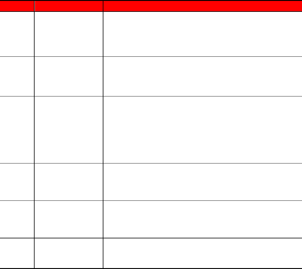
Table 4: Codes for recording the Presence of a taxon within a polygon or point

occurrence.

CODE

PRESENCE

DEFINITION

Extant

The species is known or thought very likely to occur currently in the area, which

encompasses localities with current or recent (last 20-30 years) records where

suitable habitat at appropriate altitudes remains (see note 3). Extant ranges

should be considered in the calculation of EOO. When mapping an “assisted

colonisation” it is important to note that this range should be treated as Extant.

Probably Extant

This code value has been discontinued for reasons of ambiguity. It may exist in

the spatial data but will gradually be phased out.

Possibly Extant

There is no record of the species in the area, but the species may possibly

occur, based on the distribution of potentially suitable habitat at appropriate

altitudes, although the area is beyond where the species is Extant (i.e., beyond

the limits of known or likely records), and the degree of probability of the

species occurring is lower (e.g., because the area is beyond a geographic

barrier, or because the area represents a considerable extension beyond areas

of known or probable occurrence). Identifying Possibly Extant areas is useful

to flag up areas where the taxon should be searched for. Possibly Extant ranges

should not be considered in the calculation of EOO.

Possibly Extinct

The species was formerly known or thought very likely to occur in the area

(post 1500 AD), but it is most likely now extirpated from the area because

habitat loss and/or other threats are thought likely to have extirpated the

species, and there have been no confirmed recent records despite searches.

Possibly Extinct ranges should not be considered in the calculation of EOO.

Extinct

The species was formerly known or thought very likely to occur in the area

(post 1500 AD), but it has been confirmed that the species no longer occurs

because exhaustive searches have failed to produce recent records, and the

intensity and timing of threats could plausibly have extirpated the taxon.

Extinct ranges should not be considered in the calculation of EOO.

Presence Uncertain

A record exists of the species' presence in the area, but this record requires

verification or is rendered questionable owing to uncertainty over the identity

or authenticity of the record, or the accuracy of the location. Presence

uncertain records should not be considered in the calculation of EOO.

Notes:

1. These codes are mutually exclusive, e.g. a polygon coded as “Extant” cannot also be coded as

“Extinct”.

2. In accordance with the Red List Categories and Criteria, Extant polygons can include inferred or

projected sites of present occurrence (see the Guidelines for Using the IUCN Red List Categories and

Criteria for further guidance).

3. When there is uncertainty as to whether or not a species still occurs in an area in which it was formerly

known to occur (usually because there have been no recent surveys), it is necessary for Assessors to

judge whether it is more appropriate to assign a coding of Extant or Possibly Extinct (based on

available knowledge of remaining habitat, intensity of threats, adequacy of searches, and other

evidence).

4. EOO calculations should be based on polygons coded as Extant only.

5. The old Presence code 2 (Probably Extant) is now discontinued. See section 10.1.1 for more

information

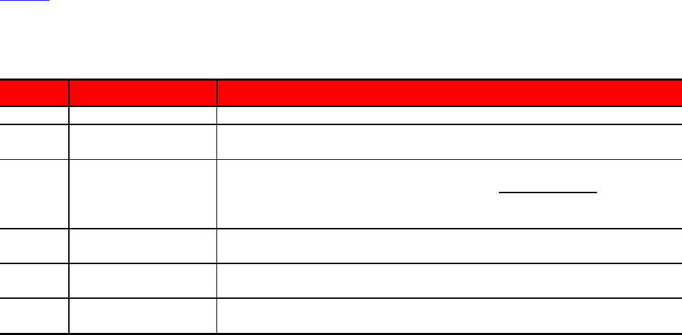
5.2 Origin Codes

Table 5 outlines the definitions for the various coding options for a taxon’s Origin within

a particular area. These Origin codes and their definitions apply to both spatial data (i.e.,

polygons and point data) and non-spatial data (e.g., Countries of occurrence in SIS)

Table 5: Codes for recording the Origin of a taxon within a polygon or point occurrence.

CODE

ORIGIN

DEFINITION

Native

The species is/was native to the area.

Reintroduced

The species is/was reintroduced within its known historical range through

either direct or indirect human activity

Introduced

The species is/was introduced outside of its known historical distribution range

through either direct or indirect human activity. Does not include species

subject to assisted colonisation. Includes species intentionally moved outside

of its native range to perform a specific ecological function.

Vagrant

The species is/was recorded once or sporadically, but it is known not to be

native to the area.

Origin Uncertain

The species’ provenance in an area is not known (it may be native,

reintroduced or introduced)

Assisted Colonisation

Species subject to intentional movement and release outside its native range

to reduce the extinction risk of the taxon.

Notes:

1. EOO estimates should be based on Origin codes 1, 2, and 6.

2. The codes are mutually exclusive, e.g. a polygon coded as Introduced cannot also be coded as

Native.

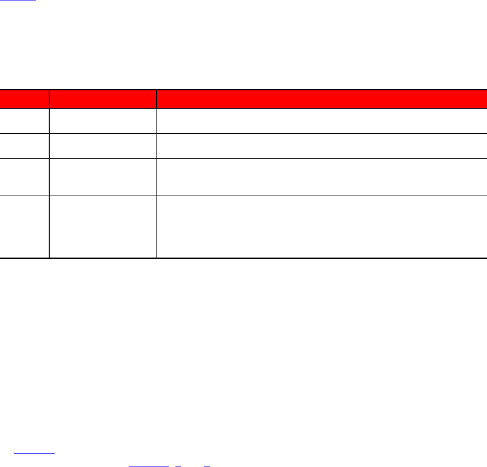
5.3 Seasonality Codes

Table 6 outlines the definitions for the various coding options for a taxon’s Seasonality

within a particular area. These Seasonality codes and their definitions apply to both

spatial data (i.e., polygons and point data) and non-spatial data (e.g., Countries of

occurrence in SIS).

Table 6: Codes for recording the Seasonality of a taxon within a polygon or point

occurrence.

CODE

SEASONALITY

DEFINITION

Resident

The species is/was known or thought very likely to be resident throughout the

year

Breeding Season

The species is/was known or thought very likely to occur regularly during the

breeding season and to breed and capable of breeding

Non-breeding Season

The species is/was known or thought very likely to occur regularly during the

non-breeding season. In the Eurasian and North American contexts, this

encompasses ‘winter’.

Passage

The species is/was known or thought very likely to occur regularly during a

relatively short period(s) of the year on migration between breeding and non-

breeding ranges.

Seasonal Occurrence

Uncertain

The species is/was present, but it is not known if it is present during part or all

of the year.

Notes:

1. ‘Regularly’ means known or thought to occur in at least 30% of years. Where it is deemed important

to record the occurrence of breeding/passage etc. for a species which occurs less often than 30% of

years (e.g. because the population is now tiny), the category can be ticked, but a comment added to

the Notes field (e.g. only recorded in 2 years during 1985-2000).

2. If the species does not regularly breed, but there are occasional breeding records, this can be noted

in the “Dist_Comm” field.

3. If there is insufficient information to be confident of assigning Non-breeding Season vs. Passage

categories, a best guess should be made, and a comment entered in the Notes field that some

ambiguity exists. Where there is extreme uncertainty, the ‘Seasonal Occurrence Uncertain’ value

should be used.

5.3.1 Presence, Origin and Seasonality quick reference

Table 7 presents a “quick reference” summary of the Presence, Origin and

Seasonality codes from Tables 4, 5 and 6.

Please note that these codes are mutually exclusive within the columns. For example,

a polygon coded as Presence “1 (Extant)” cannot also be coded as “5 (Extinct)”;

however, Presence can be coded as “1 (Extant) and Origin as “5 (Origin uncertain)”

for the same polygon.

Table 7: Summary of Presence, Origin and Seasonality codes.

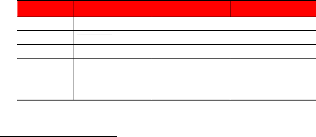
Code

Presence

Origin

Seasonality

Extant

Native

Resident

Probably Extant *

Reintroduced

Breeding season

Possibly Extant

Introduced

Non-breeding season

Possibly Extinct

Vagrant

Passage

Extinct (post 1500)

Origin uncertain

Seasonal Occurrence Uncertain

Presence uncertain

Assisted Colonisation

6 Spatial information in SIS

6.1 Countries with multiple distribution codes in the spatial data

In SIS there is only one entry recorded for each country where the taxon occurs (e.g.,

Countries of Occurrence (COO)). However, since it can happen that within a country

there are multiple polygons or points with different distribution codes, it is important

that the appropriate corresponding code is captured for the non-spatial data. Below are

the rules to guide this coding to ensure correspondence between the spatial and non-

spatial data.

● Presence codes ( > means has precedence over):

1. Extant > 3. Possibly Extant > 4. Possibly Extinct > 5. Extinct > 6. Presence

Uncertain

● Origin codes:

1. Native > (2. Reintroduced / 6. Assisted Colonisation) > 3. Introduced > 4.

Vagrant > 5. Origin Uncertain

For example, if a taxon has two polygons (A and B) for Country X, where polygon A is

coded as Presence 1 and Origin 5, and polygon B is coded as Presence 3 and Origin 3,

then when recording the COO for Country X, Presence should be 1 and Origin should

be 3.

Note that in recording Countries of Occurrence in SIS, it is possible for a country to

have multiple subcountries which may have different Presence, Origin and Seasonality

codes. The same rules as above apply. For example, if a taxon occurs in two subcountries

(A and B) for Country X, where subcountry A is coded as Presence 1 and Origin 5, and

subcountry B is coded as Presence 3 and Origin 3, then when recording the COO for

Country X, Presence should be 1 and Origin should be 3.

7 Extent of occurrence (EOO), area of occupancy (AOO)

7.1 Extent of occurrence (EOO)

Extent of occurrence (EOO) is defined as "the area contained within the shortest

continuous imaginary boundary which can be drawn to encompass all the known,

inferred or projected sites of present occurrence of a taxon, excluding cases of

vagrancy".

EOO is a parameter that measures the spatial spread of the areas currently occupied by

the taxon. It is included in the IUCN Red List Criteria as a measure of the degree to

which risks from threats are spread spatially across the taxon’s geographical distribution

(see section 4.9 of the Red List Guidelines).

7.1.1 How should EOO be calculated for polygon maps and point maps?

EOO should be calculated by applying a Minimum Convex Polygon (MCP) (the

smallest polygon in which no internal angle exceeds 180 degrees and which contains

all the sites of occurrence) around the mapped range, which should be mapped as

accurately as possible based on all of the available data.

More information on EOO can be found in Joppa, L. N., Butchart, S. H. M.,

Hoffmann, M., Bachman, S. P., Akçakaya, H. R., Moat, J. F., Böhm, M., Holland, R.

A., Newton, A., Polidoro, B. and Hughes, A. 2016. Impact of alternative metrics on

estimates of extent of occurrence for extinction risk assessment. Conservation

Biology 30: 362–370. doi:10.1111/cobi.12591.

Exceptions will not be allowed for taxa with:

1. 'Doughnut distributions' e.g., aquatic species confined to the margins of a lake.

(Such distributions should reduce not increase extinction risk for threats that

are also restricted to similar distributions).

2. Small and highly disjunction subpopulations (e.g., for which the majority of

the population occurs on a mainland with an additional subpopulation on a

small and distant island, the inclusion of which within the MCP would

considerably increase the EOO estimate). Note this contradicts what is stated

in the Mace et al. (2008) paper.

3. Curved linear distributions that are shaped in an arc. (Most of the increase in

EOO estimate for such taxa would be as a result of joining up the various

"blobs" into a single polygon, rather than from including the area within the

inside of the curve).

In the case of migratory species, EOO should be based on the minimum of the

breeding or nonbreeding (wintering) areas, but not both, because such species are

dependent on both areas, and the bulk of the population is found in only one of these

areas at any time. If EOO is less than AOO, EOO should be changed to make it equal

to AOO to ensure consistency with the definition of AOO as an area within the EOO.

For more information on EOO, see section 4.9 in the Red List Guidelines.

The IUCN Red List EOO Calculator tool, which runs in ArcGIS, (downloadable from

the IUCN Red List Spatial Resources page on the IUCN Red List website) calculates

EOO using only polygons and points of Presence 1 (Extant) and Origin 1 or 2 (Native

and Re-Introduced), and it does so separately for Seasonality codes 1 and 2 (if

present) or 1 and 3 (if present), with EOO being taken as the lower of these two

values.

Area or geometry calculations is recommended be performed in Cylindrical Equal

Area (world) projection (but other projections can also be used if they provide better

results e.g. for specific locations)

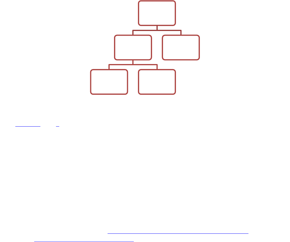
Figure 1: Schematic representation of polygon coding and calculation of

EOO.

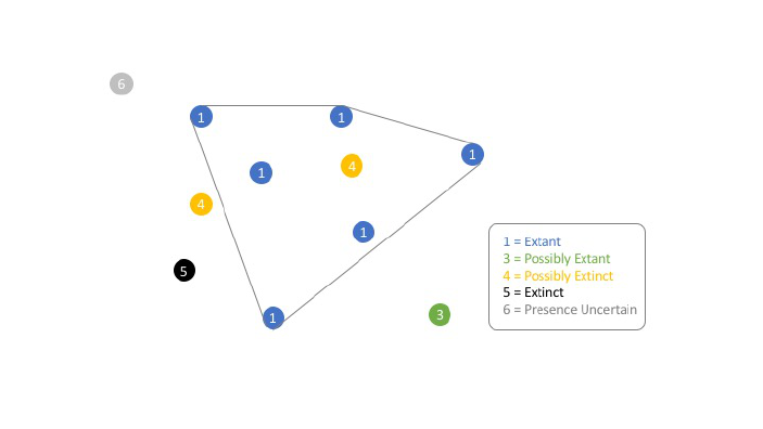
Figure 2: Schematic representation of point coding and calculation of

EOO.

7.2 Area of occupancy (AOO)

Area of occupancy (AOO) is a scaled metric that represents the area of suitable habitat

currently occupied by the taxon. Area of occupancy is included in the IUCN Red List

Criteria for two main reasons:

1. AOO is a measure of the ‘insurance effect,’ whereby taxa that occur within

many patches or large patches across a landscape or seascape are ‘insured’

against risks from spatially explicit threats. In such cases, there is only a small

risk that the threat will affect all occupied patches within a specified time

frame. In contrast, taxa that occur within few small patches are exposed to

elevated extinction risks because there is a greater chance that one or few

threats will affect all or most of the distribution within a given time frame.

2. There is generally a positive correlation between AOO and population size.

AOO can therefore be a useful metric for identifying species at risk of

extinction because of small population sizes when no data are available to

estimate population size and structure.

To ensure valid use of the criteria and maintain consistency of Red List assessments

across taxa it is essential to scale estimates of AOO using 2 x 2 km grid cells. Estimates

of AOO are highly sensitive to the spatial scale at which AOO is measured. Thus, it is

possible to arrive at very different estimates of AOO from the same distribution data if

they were calculated at different scales. The thresholds of AOO that delineate different

categories of threat in criteria B2 and D2 are designed to assess threats that affect areas

in the order of 10-2,000 km², and therefore assume that AOO is estimated at a particular

spatial scale. The Red List Guidelines require that AOO is scaled using 2 x 2 km grid

cells (i.e., with area of 4 km²) to ensure that estimates of AOO are commensurate with

the implicit scale of the thresholds. Use of the smallest available scale (finest grain) to

estimate AOO (sometimes erroneously called "actual area" or "actual AOO") is not

permitted, even though mapping a species' distribution at the finest scale may be

desirable for purposes other than calculating AOO. Habitat maps with higher resolutions

can be used for other aspects of a Red List assessment, such as calculating reduction in

habitat quality as a basis of population reduction for criterion A2(c) or estimating

continuing decline in habitat area for B2(b), as well as for conservation planning.

For more information on AOO, see section 4.10 in the Red List Guidelines.

8 Generating a distribution map

8.1 Software and formats

There are several ways in which maps can be generated, and the preference is always to

generate digital maps (i.e., maps in the form of Shapefiles, or KML or ESRI File

Geodatabase etc…). There is a suite of software which can be used to do this, namely:

1. ArcGIS desktop – licensed software. IUCN can provide a license for this under

strict terms of use (contact the IUCN Red List for further information), provided

Figure 3: Two examples of the distinction

between extent of occurrence and area of

occupancy; (A) is the spatial distribution

of known, inferred or projected sites of

occurrence, (B) shows one possible

boundary to the extent of occurrence,

which is the measured area within this

boundary, (C) shows one measure of area

of occupancy which can be measured by

the sum of the occupied grid squares.

the software is being used for the assessment of a taxon, or for such similar

purpose.

2. QGIS – free open-source software

3. Google Earth Pro – free software.

4. Google My Maps in Google Drive – free software.

The IUCN Red List Unit and Red List Partners have developed a series of tools to make

the mapping process easy for Assessors. These resources can be found on the IUCN

Spatial Data Resources page on the IUCN Red List website.

8.2 Tools

The IUCN Spatial Data Resources page on the IUCN Red List website provides access

to a range of tools to help you to create distribution maps for taxa being assessed for

The IUCN Red List. Some important tools worth mentioning here are:

● RedList Toolbox: This is designed for use with ArcGIS Desktop, and includes

documentation to help Assessors generate a digital map in the appropriate format

and structure.

● GeoCAT: RBG Kew developed this free, online tool to allow users to create

maps using point data. It supports the IUCN Points standards, and also includes

tools that automatically calculate EOO and AOO (based on the point data).The

polygons from GeoCAT are not suitable as maps.

● IUCN Red List Mapping Tool (Freshwater species): This free, online

mapping tool was developed for creating distribution maps for inland water

species. It is integrated with SIS (i.e., it links to taxa within existing working sets

in SIS) and it includes HydroBASINs, allowing users to map to those areas.

Please contact the Freshwater Biodiversity Unit for more information.

8.3 Standard GIS layers / basedata

A recommended list of GIS layers (or ‘spatial basedata’) is available for Assessors to

use when they are creating distribution maps. These layers include, for example, the

Country layer, which should be used as the base-layer for mapping taxa to countries. It

is important that Assessors use these recommended spatial data layers (basedata maps)

to ensure that the generated maps comply with other tools within the Red List, and also

to standardize the maps displayed on the IUCN Red List.

More information on these base-layers can be found on the IUCN Spatial Data

Resources page on the IUCN Red List website.

These base-layers may change, or decisions may be taken by the IUCN SSC Red List

Technical Working Group to recommend different base-layers; therefore, it is strongly

recommended that Assessors check the IUCN Red List website for current guidance and

information.

8.4 Mapping consistency

The following recommendations are provided to ensure consistency between taxa being

mapped:

1. How to convert points to polygon ranges: due to the nature of a taxon it is at the

expert’s discretion to decide on the method of creating a polygon from points, if

they would like to do it. Some suggestions (they can be used singly or in

combination) are:

a) Buffering the points to a taxon’s appropriate range. For example,

consideration of the taxon’s life history, such as roaming range, feeding

range, breeding or migration.

b) Using habitat as a guide to map to known areas around the points.

c) Using spatial data from other ranges of other taxa, for example a prey or

host species.

d) Bathymetry and altitude selection. Note that raster files cannot be

submitted but conversion from raster to polygon is possible in ArcMap and

QGIS software.

2. Overlapping polygons within a taxon’s range: whilst it is entirely feasible for a

species to have overlapping polygons with different attributes (e.g. Presence,

Origin, different citations, etc…), it is important to ensure that this is actually

really the case, and not a mistake during the mapping process. In order to prevent

discrepancies, check whether the polygons overlap each other in joining areas. A

taxon’s subspecies, varieties and subpopulations within the taxon’s range may

overlap. Overlapping polygons can introduce geometry challenges, including

during analysis.

3. Mapping subspecies, varieties and subpopulations: when mapping subspecies,

varieties and subpopulations these ranges should be included within the species

polygon.

4. Restricted ranges: when mapping to a small area, such as a cave, small

HydroBASIN or island it is import to keep in mind the scope of the taxon and its

habitat and ecology, while not generalizing the range as this may inflate the

Minimum Convex Polygon (MCP) and change the extent of occurrence. For

inland water assessments, as with other groups, the map should represent the best

possible representation of the distribution. For those inland water taxa with

distributions more restricted than the finest scale HydroBASINs layer, the range

should be mapped as a polygon reflecting e.g., the location of a cave or small

wetland to which a taxon is restricted, rather than generalising to finest scale

HydroBASIN layer.

5. Island taxa: When a taxon is present on an island it is important to state the island

in the attributes due to organisations using different global country base layers in

which some may not have the island you have selected.

6. Marine taxa: Due to the dynamic nature of the marine biome it is important to

take bathymetry into account. Bathymetry ranges, like those in the habitat

classification scheme, can be found on the Spatial Data Resources page. If for

example, a taxon is found between 5-20 m depth then the polygon can be clipped

to the 25 m bathymetry and the 5 m bathymetry can be erased.

7. Projections: Each taxon’s spatial data is required to be projected (i.e., to a set

coordinate system). This enables the taxon’s spatial data to be applied to other

spatial datasets for integration and storage. The recommended projection for the

IUCN Red List is WGS84. To check the projection of a file go to the files

properties in ArcMap and check the Source tab. If the “Geographic Coordinate

System” says <Undefined>, you can use the Define Projection (Data

Management) tool. If the “Geographic Coordinate System” is something other

than the WGS_1984 projection you can convert it using the Project tool.

8. Smoothing: Smoothing a polygon removes sharp angles in the polygon and is

used for aesthetic and visual reasons. If this tool is used, please ensure that it does

not affect the coverage of the taxon’s spatial range.

For tools, general guidance and information on best practices for mapping ranges please

refer to the IUCN Red List Spatial Data Resources page.

8.5 Sensitive species guidelines

A taxon’s map will not be shown or made publicly available when the data_sens field

contains a ‘Y’ (this means that the specific taxon polygon is marked as being sensitive).

Information on why this polygon or point is sensitive should be recorded in the

sens_comms attribute (see table 2). A generalized polygon may be used instead; there

are two methods to consider depending on the situation:

● Buffer: a buffer of a minimum of 10 km when more than one point is available

(the buffer distance can be larger, e.g. the range could be mapped to country-

level).

● Irregular polygon: if only one point is provided then a round buffer would show

the species to be in the centre. An irregular shaped polygon would therefore

show approximately where the taxon is distributed but generalized enough to

avoid giving away its exact location.

For further details see the IUCN Red List policy on Sensitive Data Access Restrictions.

9 What will happen to your map data?

Once distribution map data have been checked and processed, and are part of assessments

that are being published on the IUCN Red List, the data are used in the following way:

● Points and polygons are displayed on the IUCN Red List website, via the Map

Browser, which is an interactive tool.

o There is a map icon on every taxon page on the IUCN Red List website,

which opens the Map Browser.

o The spatial data is projected to WGS84/ Mercator for display on the map.

● Points and polygons are used to determine EOO – using an MCP around the

points/polygons.

● The points and polygons are used to generate images of the maps, using the Map

Batcher, which presents them in a format for use in workshops, presentations, the

PDFs of the assessments, etc.

● The data are also submitted to Integrated Biodiversity Assessment Tool (IBAT):

IBAT provides a basic risk screening on biodiversity. It draws together information

on globally recognised biodiversity information drawn from a number of IUCN’s

Knowledge Products. The IUCN Red List of Threatened Species data are provided

in a hexagonal grid format, as well as a full download of the spatial data depending

on type of user access.

● Spatial data are made available for download individually, in bulk, or via an API

for non-commercial use.

● Used in data analysis e.g. species richness maps, climate change vulnerability

projections. In such circumstances, the spatial data used should be referenced and

also credited appropriately.

● The Country of occurrence is not displayed in map, but is published in the taxon’s

fact sheet on the Red List

● Maps that are marked as Sensitive in the map file data (i.e. data_sens field is TRUE)

are not displayed on the IUCN Red List website, or made available, unless special

permission has been granted.

● The data are also made available through an API (which is an interface through

which the Red List data can be queried and used programmatically). Access to the

API is granted through a token, to provide some level of control.

9.1 Countries of occurrence (COO) data

Countries of occurrence (COO) information is displayed on the IUCN Red List website.

This information is used to support the website’s functionality (especially country

searches) and to allow basic analyses (e.g., endemism).

9.2 Legend combinations from distribution codes

Different combinations of the Presence, Origin and Seasonality codes are used to create

legends for the final distribution map.

The list of distribution codes used for the legends can be found on the Spatial Data

Resources page on the IUCN Red List website.

10.0 Updates regarding Spatial Data

10.1 Presence Codes (last updated 2014)

Presence codes updated with new definitions. Data prior to this change will remain and

updated as re-assessments take place.

10.1.1 Implications of updated Presence for existing spatial data

Some distribution maps published on the IUCN Red List were created using a

previous version of the Presence codes. The implications of the current Presence

codes (as defined in Table 4) on existing spatial data that have not been migrated yet

are outlined below.

1. All polygons or points currently coded using the old Presence 2 (Probably

Extant) should be recoded as Presence 1 (Extant).

2. For inland water taxa:

(i) HydroBASINs coded as Presence 2 should be recoded as Presence 1

if they fall within an MCP drawn around all existing Presence 1s, or

as Presence 3 (Possibly Extant) if they fall outside of this MCP.

(ii) If all HydroBASINS in the map are coded as Presence 2 (e.g., where

point locality data are unavailable and distributions have been

inferred), you will need to decide which Presence code (1 or 3) is

appropriate for occurrence of the taxon in each of these areas. Please

note that if Presence 3 is used for all HydroBASINs on the map, this

may have consequences for the taxon’s Red List assessment (e.g.,

EOO cannot be calculated if no records exist for the taxon, which will

affect any taxa currently assessed under criterion B1); in such cases a

reassessment will be required.

If unsure about the above, please contact the Red List Unit for further

clarification.

3. Some polygons or points currently coded as 3 may need review to see whether

they should be recoded as 1 (because they may actually represent inferred or

projected sites of occurrence). This would not affect EOO estimation if such

records are within the current MCP, but obviously would if such records fall

beyond the current MCP.

4. Some polygons or points currently coded as Presence 6 (Presence Uncertain)

may need to be reassigned to 1 or 4 (see Note 3 attached to Table 4)

See Figures 1 and 2 in section 7.0 for more information on recoding Presence codes

and on using the Presence codes for EOO calculations.

10.2 Origin code Assisted Colonisation (last updated 2016)

New Origin code (6) added for species subject to intentional movement and release

outside its native range to reduce the extinction risk of the taxon.

10.3 Legend Update (last updated 2016)

The legend was improved to contain all the values for Presence, Origin and Seasonal.

The new list can be found on the IUCN Red List Spatial Resources page. Previously, all

the different legends (or distribution codes combinations) were not being displayed on

the website, but now, they all are.

11 Abbreviations, acronyms and definitions

AOO: Area of occupancy. A parameter used in the IUCN Red List Categories and Criteria

to measure the area within the 'extent of occurrence' which is occupied by a taxon,

excluding cases of vagrancy (see section 4.10 of the Red List Guidelines).

Assisted colonisation: The intentional movement and release of an organism outside its

indigenous range to avoid extinction of populations of the focal taxon. Within the mapping

process, the assisted colonisation range should be coded in the attributes as Extant

(Presence = Extant, Origin = Assisted Colonisation).

EOO: Extent of occurrence. A parameter used in the IUCN Red List Categories and

Criteria to measure the spatial spread of the areas currently occupied by the taxon (see

section 4.9 of the Red List Guidelines).

MCP: Minimum Convex polygon. This is the smallest polygon in which no internal angle

exceeds 180 degrees and which contains all sites of known, inferred and projected

occurrence.

Polygon: A map feature that bounds an area at a given scale, such as a country on a world

map or a district on a city map.

Projection: A projection uses the datum as a point of reference, it's location on Earth.

In GIS, there are two types of "coordinate systems": Geographic Coordinate System: a

georeference or location of the map on the globe and Projected Coordinate System: how

the map is displayed. The standard Geographical Coordinate System the IUCN Red List

uses is WGS 1984.